7 Appendix
The appendix walks through all of the code performed in this project including data wrangling, feature extraction, and model fitting.
7.1 Data Wrangling/Feature Extraction
7.1.1 Basic Data Wrangling
We begin by reading in our raw data:
politifact_df_raw <- read_csv("../data-raw/politifact_phase2_clean_2018_7_3.csv") We then clean up the raw data by getting rid of rows with duplicate URLs, getting rid of targets we don’t care about, and creating two columns for our targets (one numerical, one categorical) since different models require different variable types for target values. In addition, we create a unique ID for each row (which consists of an article’s claim and its PolitiFact truth rating).
# clean up raw data
politifact_df_cleaned <- politifact_df_raw %>%
  # get rid of duplicate URLs (reasoning for this is discussed in limitations)
  distinct(politifact_url_phase1, .keep_all = TRUE) %>%
  # keep only the two targets we care about
  filter(fact_tag_phase1 == "True" | fact_tag_phase1 == "Pants on Fire!") %>%
  # change desired targets to categorical and numerical
  mutate(targets_numerical = as.numeric(ifelse(fact_tag_phase1 == "True", 1, 0)),
         targets_categorical = as.factor(ifelse(fact_tag_phase1 == "True", 1, 0))) %>%
  # rename the article claim variable
  rename(article_claim = article_claim_phase1) %>%
  # only keep the variables we care about
  select(article_claim, targets_numerical, targets_categorical)

# add an id
politifact_df_cleaned$article_id <- seq.int(nrow(politifact_df_cleaned))
# take a look at our cleaned dataframe
glimpse(politifact_df_cleaned)
## Rows: 1,911
## Columns: 4
## $ article_claim <chr> "\"When you tally up their representation in Congress and governorships…
## $ targets_numerical <dbl> 1, 0, 0, 0, 1, 0, 1, 0, 1, 0, 1, 1, 0, 0, 1, 0, 0, 1, 0, 0, 1, 0, 0, 0,…
## $ targets_categorical <fct> 1, 0, 0, 0, 1, 0, 1, 0, 1, 0, 1, 1, 0, 0, 1, 0, 0, 1, 0, 0, 1, 0, 0, 0,…
## $ article_id <int> 1, 2, 3, 4, 5, 6, 7, 8, 9, 10, 11, 12, 13, 14, 15, 16, 17, 18, 19, 20, …7.1.2 Cleaning the Text/Reducing the Vocabulary Size
Since the article_claim column contains messy text data, text cleaning is needed.
The text cleaning done in this project consists of the following: removing punctuation, making all
letters lowercase, removing English stop words, lemmatizing each word, removing numbers, and
removing any extra white space. Removing stop words, numbers, and lemmatizing words all leads to a
decrease in the size of the overall vocabulary (all unique words across a set of text).
The clean_text function performs the aforementioned text cleaning and vocabulary
reduction:
# a function to perform text cleaning
clean_text <- function(input_text) {
  # remove punctuation
  output_text <- removePunctuation(input_text) %>%
    # make all letters lowercase
    tolower() %>%
    # remove a custom list of English stop words (from the `tm` package)
    removeWords(stopwords("en")) %>%
    # lemmatize the words in the text
    lemmatize_strings() %>%
    # remove any numbers in the text
    removeNumbers() %>%
    # get rid of any extra white space
    stripWhitespace()

  return(output_text)
}

# an example of using the `clean_text` function
clean_text("'Trump approval rating    better than Obama  and Reagan at
            same point in their presidencies.'")
## [1] "trump approval rate good obama reagan point presidency"The clean_text function is used to clean up the text in
politifact_df_cleaned.
# clean up the article claim text, create a final dataframe
politifact_df_final <- politifact_df_cleaned %>%
  mutate(article_text = clean_text(article_claim)) %>%
  select(article_id, article_text, targets_numerical, targets_categorical)

glimpse(politifact_df_final)
## Rows: 1,911
## Columns: 4
## $ article_id <int> 1, 2, 3, 4, 5, 6, 7, 8, 9, 10, 11, 12, 13, 14, 15, 16, 17, 18, 19, 20, …
## $ article_text <chr> "tally representation congress governorship democrat almost low represe…
## $ targets_numerical <dbl> 1, 0, 0, 0, 1, 0, 1, 0, 1, 0, 1, 1, 0, 0, 1, 0, 0, 1, 0, 0, 1, 0, 0, 0,…
## $ targets_categorical <fct> 1, 0, 0, 0, 1, 0, 1, 0, 1, 0, 1, 1, 0, 0, 1, 0, 0, 1, 0, 0, 1, 0, 0, 0,…7.1.3 Train/Test Split
In order to evaluate classification models, a training set and a testing set are needed. In this project, an \(80%\)/\(20%\) training/testing split is used.
# set the seed to ensure reproducibility
set.seed(2)

# the number of rows in our final data frame
num_politifact_rows <- nrow(politifact_df_final)

# get random row numbers from our data frame (80% of all possible row numbers
# will be stored in `random_row_numbers` since we have an 80/20 split)
random_row_numbers <- sample(1:num_politifact_rows, 0.8 * num_politifact_rows)

# use our randomly generated row numbers to select 80% of our data for training
politifact_df_train  <- politifact_df_final[random_row_numbers, ] %>%
  # sort by article id
  arrange(article_id)
# and use the remaining 20% of our data for testing
politifact_df_test   <- politifact_df_final[-random_row_numbers, ] %>%
   arrange(article_id)

# keep track of our target variables in a list
train_targets_numerical <- politifact_df_train$targets_numerical
train_targets_categorical <- politifact_df_train$targets_categorical

test_targets_numerical <- politifact_df_test$targets_numerical
test_targets_categorical <- politifact_df_test$targets_categorical
We next want to make sure our training/testing split has a roughly equal distribution of each target value.
prop.table(table(train_targets_numerical))## train_targets_numerical
## 0 1
## 0.4443717 0.5556283prop.table(table(test_targets_numerical))## test_targets_numerical
## 0 1
## 0.4830287 0.5169713Across our two target variables—where a “false” piece of news corresponds to \(0\) and a “true” piece of news corresponds to \(1\)—we observe a \(44.4%\), \(55.6%\) to \(48.3%\), \(51.7%\) training/testing split. Since the proportion of target values is reasonably even, we can proceed with this split.
7.1.4 Creating a Document Term Matrix
To create a Document Term Matrix (DTM), the article_text needs to be tokenized into
individual words so that an overall vocabulary can be created. Here n-grams are used (from \(n=1\) to \(n=3\)). This means that
all possible \(1\), \(2\), and
\(3\) word combinations are included in the vocabulary. Note that
we must create our vocabulary using only the training data, since our test data should not be
looked at until model evaluation.
Once a vocabulary is created, terms that only appeared once throughout our training dataset are removed. This reduces the size of the vocabulary terms from \(28678\) terms to \(806\), which is a far more manageable number of terms to have in a DTM.
# tokenize the text into individual words
tokenizer_train <- word_tokenizer(politifact_df_train$article_text) %>%
  itoken(ids = politifact_df_train$article_id, progressbar = FALSE)

# this test tokenizer will be used later
tokenizer_test <- word_tokenizer(politifact_df_test$article_text) %>%
  itoken(ids = politifact_df_test$article_id, progressbar = FALSE)

# create our vocabulary with the training data
vocabulary <- create_vocabulary(tokenizer_train, ngram = c(1L, 3L))
# we observe 28678 unique terms, this is too large
nrow(vocabulary)
## [1] 28678# prune our vocabulary to only include terms used at least 2 times
pruned_vocabulary <- prune_vocabulary(vocabulary, term_count_min = 5)
# we now observe 806 unique terms, which is more manageable
pruned_vocabulary## Number of docs: 1528
## 0 stopwords: ...
## ngram_min = 1; ngram_max = 3
## Vocabulary:
## term term_count doc_count
## 1: account 5 5
## 2: affair 5 5
## 3: affect 5 4
## 4: africanamerican 5 5
## 5: agree 5 5
## ---
## 802: percent 130 102
## 803: obama 131 130
## 804: year 149 130
## 805: state 171 159
## 806: say 417 372Now that we have a reasonably sized vocabulary, we can create our training and testing DTMs.
# create our training and testing DTMs using our tokenizers
vocabulary_vectorizer <- vocab_vectorizer(pruned_vocabulary)

dtm_train <- create_dtm(tokenizer_train, vocabulary_vectorizer)
dtm_test <- create_dtm(tokenizer_test, vocabulary_vectorizer)
We then change our DTMs to hold term frequency–inverse document frequency (tf-idf) values, which will normalize the DTMs and increase the weight of terms which are specific to a single document (or handful of documents) and decrease the weight for terms used in many documents.27
tfidf <- TfIdf$new()

# fit model to train data and transform train data with fitted model
dtm_train <-  fit_transform(dtm_train, tfidf)
dtm_test <-  fit_transform(dtm_test, tfidf)

# convert our DTMs to a matrix and data frame--different formats are needed
# for different models (`keras` only takes matrices for example)
dtm_train_matrix <- as.matrix(dtm_train)
dtm_test_matrix <- as.matrix(dtm_test)

dtm_train_df <- as.data.frame(dtm_train_matrix)
dtm_test_df <- as.data.frame(dtm_test_matrix)
The data wrangling and feature extraction is now complete. Our features exist in the form of Document Term Matrices where each column represents a term, each row represents a PolitiFact article, and each cell holds the term frequency–inverse document frequency value of that term. Our targets exist as \(0\)’s and \(1\)’s, where a “false” piece of news corresponds to 0 and a “true” piece of news corresponds to 1. We observe a small portion of our training and testing DTMs below. Note that each value is \(0\) since our vocabulary contains \(3000\) terms and it is very unlikely that the first \(5\) terms are in any of the \(10\) different rows we are looking at.
dtm_train_df[1:5, 1:5]## account affair affect africanamerican agree
## 1 0 0 0 0 0
## 3 0 0 0 0 0
## 6 0 0 0 0 0
## 8 0 0 0 0 0
## 9 0 0 0 0 0dtm_test_df[1:5, 1:5]## account affair affect africanamerican agree
## 2 0 0 0 0 0
## 4 0 0 0 0 0
## 5 0 0 0 0 0
## 7 0 0 0 0 0
## 12 0 0 0 0 07.2 Initial Model Fitting
This section displays the code for each of the initial models fit in an attempt to classify fake news.
7.2.1 Naive Bayes
We can use the e1071 package to run a Naive Bayes model. Note that the
e1071::naiveBayes function requires categorical targets and accepts features in the
form of a dataframe.
# applying Naive Bayes model to training data
nb_model <- e1071::naiveBayes(x = dtm_train_df, y = train_targets_categorical,
                              laplace = 1)

# predicting applying to test set
nb_predicted_values <- predict(nb_model, dtm_test_df)

nb_confusion_matrix <- caret::confusionMatrix(nb_predicted_values,
                                              test_targets_categorical,
                                              dnn = c("Predicted", "Actual"))
# confusion matrix table
nb_confusion_matrix$table
## Actual
## Predicted 0 1
## 0 137 104
## 1 48 94# 60.3% accuracy
round(nb_confusion_matrix$overall[1], 3)## Accuracy
## 0.603# [55.2%, 65.2%] 95% CI for accuracy
round(nb_confusion_matrix$overall[3:4], 3)## AccuracyLower AccuracyUpper
## 0.552 0.652# for full information, uncomment and run the following line of code:
# nb_confusion_matrixOur Naive Bayes model performs rather poorly with an accuracy of only \(60.3\%\) (and a 95% confidence interval of \([55.2\%, 65.2\%]\)).
7.2.2 Basic Logistic Regression
Since the glm function requires a formula, we must create a new dataframe combining
our features and targets. Note that the glm function requires categorical targets.
# logistic regression data frames (training and testing)
lr_df_train <- cbind(dtm_train_df, train_targets_categorical)
lr_df_test <- cbind(dtm_test_df, test_targets_categorical)
We now fit the logisitic regression model and calculate its accuracy.
# fit the basic logistic regression model
blr_model <- glm(train_targets_categorical ~ ., data = lr_df_train,
                           family = binomial(link = "logit"))

# calculated the predicted value probabilities (which gives us
# the probability that an observation is classified as 1)
blr_predicted_value_probs <- predict(blr_model, newdata = lr_df_test,
                                 type = "response")

# turn the probabilites into 1's or 0's--if the probability of being a 1
# is greater than 50%, turn it into a 1 (turn it into a 0 otherwise)
blr_predicted_values <- as.factor(ifelse(blr_predicted_value_probs > 0.5, 1, 0))

blr_confusion_matrix <- caret::confusionMatrix(blr_predicted_values,
                                               test_targets_categorical,
                                               dnn = c("Predicted", "Actual"))

# confusion matrix table
blr_confusion_matrix$table
## Actual
## Predicted 0 1
## 0 102 63
## 1 83 135# 61.9% accuracy
round(blr_confusion_matrix$overall[1], 3)## Accuracy
## 0.619# [56.8%, 66.8%] 95% CI for accuracy
round(blr_confusion_matrix$overall[3:4], 3) ## AccuracyLower AccuracyUpper
## 0.568 0.668Our basic logistic regression model performs rather poorly with an accuracy of only \(61.9\%\) (and a 95% confidence interval of \([56.8\%, 66.8\%]\)).
7.2.3 Logistic Regresion with L1 penalty (Lasso Regression)
This model is an improved form of logistic regression using an L1 regularization penalty and
5-fold cross-validation using the glmnet package. Logistic regression using an L1
regularization is also known as “Lasso regression.” Lasso regression shrinks the less important
features’ coefficients to zero, thus removing some features altogether.28 This works well for feature selection when
there are a large number of features, as in our case (we have \(806\) features).
N-fold cross-validation (here \(n=5\)) is used to “flag problems like overfitting or selection bias and to give an insight on how the model will generalize to an independent dataset.”29
The cv.glmnet function from the glmnet function is used here to perform
the Lasso regression and 5-fold cross-validation discussed above. Note that our features must be
in the form of a matrix here (not a dataframe) and our targets must be numerical.
num_folds <- 5
threshold <- 1e-4
max_num_it <- 1e5

# manually compute our folds so below model doesn't vary each time it's run
set.seed(2)
fold_id <- sample(rep(seq(num_folds), length.out = nrow(dtm_train_matrix)))

# use cross validation to determine the optimal lambda value for L1 penalty
lasso_model <- cv.glmnet(x = dtm_train_matrix, y = train_targets_numerical,
                              # this gives us logistic regression
                              family = "binomial",
                              # L1 penalty
                              alpha = 1,
                              # interested in the area under the ROC curve
                              type.measure = "auc",
                              # 5-fold cross-validation
                              nfolds = num_folds,
                              # manually create our folds for reproducibility
                              foldid = fold_id,
                              # a higher threshold is less accurate,
                              # but has faster training
                              thresh = threshold,
                              # a lower number of iterations is less accurate,
                              # but has faster training
                              maxit = max_num_it)

lasso_predicted_value_probs <- predict(lasso_model, dtm_test_matrix,
                                       type = "response")

lasso_predicted_values <- as.factor(ifelse(lasso_predicted_value_probs > 0.5, 1, 0))

lasso_confusion_matrix <- caret::confusionMatrix(lasso_predicted_values,
                                                 test_targets_categorical,
                                                 dnn = c("Predicted", "Actual"))

# confusion matrix table
lasso_confusion_matrix$table
## Actual
## Predicted 0 1
## 0 91 22
## 1 94 176# 69.7% accuracy
round(lasso_confusion_matrix$overall[1], 3)## Accuracy
## 0.697# [64.8%, 74.3%] 95% CI for accuracy
round(lasso_confusion_matrix$overall[3:4], 3) ## AccuracyLower AccuracyUpper
## 0.648 0.743Our logistic regression model using an L1 regularization penalty performs significantly better than our basic logistic regression model. This logistic regression model has an accuracy of \(69.7\%\) (and a 95% confidence interval of \([64.8\%, 74.3\%]\)).
7.2.4 Support Vector Machine
We can use the e1071 package to run a Support Vector Machine (SVM). Note that the
randomForest function requires categorical targets and accepts features in the form
of a dataframe.
svm_model <- e1071::svm(x = dtm_train_df, y = train_targets_categorical,
                        type = "C-classification", kernel = "sigmoid")

svm_predicted_values <- predict(svm_model, dtm_test_df)

svm_confusion_matrix <- caret::confusionMatrix(svm_predicted_values,
                                               test_targets_categorical,
                                               dnn = c("Predicted", "Actual"))

# confusion matrix table
svm_confusion_matrix$table
## Actual
## Predicted 0 1
## 0 113 46
## 1 72 152# 69.2% accuracy
round(svm_confusion_matrix$overall[1], 3)## Accuracy
## 0.692# [64.3%, 73.8%] 95% CI for accuracy
round(svm_confusion_matrix$overall[3:4], 3) ## AccuracyLower AccuracyUpper
## 0.643 0.738Our SVM performs reasonably well with an accuracy of \(69.2\%\) (and a 95% confidence interval of \([64.3\%, 73.8\%]\)).
7.2.5 Random Forest
We can use the randomForest package to run a Naive Bayes model. Note that the
randomForest function requires categorical targets and accepts features in the form
of a dataframe.
set.seed(2)
rf_model <- randomForest(x = dtm_train_df, y = train_targets_categorical)
rf_predicted_values <- predict(rf_model, dtm_test_df)

rf_confusion_matrix <- caret::confusionMatrix(rf_predicted_values,
                                              test_targets_categorical,
                                              dnn = c("Predicted", "Actual"))

# confusion matrix table
rf_confusion_matrix$table
## Actual
## Predicted 0 1
## 0 124 51
## 1 61 147# 70.8% accuracy
round(rf_confusion_matrix$overall[1], 3)## Accuracy
## 0.708# [65.9%, 75.3%] 95% CI for accuracy
round(rf_confusion_matrix$overall[3:4], 3) ## AccuracyLower AccuracyUpper
## 0.659 0.753Our random forest model performs reasonably well with an accuracy of \(70.8\%\) (and a 95% confidence interval of \([65.9\%, 75.3\%]\)).
7.3 Deep Learning Model Fitting
This section displays the code for the deep learning models fit in an attempt to classify fake news.
7.3.1 Multilayer Perceptron Neural Network
The keras package is used to fit a Multilayer Perceptron (MLP). Here, a MLP with one
input layer, one hidden layer, and one output layer is created. The keras requires
features to be stored in matrices and targets to be numerical.
Note that the keras package randomizes initial weights each time a model is run,
meaning that results will vary slightly each time the following two code chunks are run
(specifically, Figure 7.1 will change and the MLP
model’s accuracy will change). The provided function to ensure reproducibility in
keras(which is named use_session_with_seed()) does not currently work
within a knitted R Markdown file. Additionally, using the normal set.seed() function
does not alleviate the issue. For a more detailed breakdown, I’ve created a file outlining the
problem that can be found in the directory scratch-work/keras-reprex.R.
set.seed(2)
num_features <- ncol(dtm_train_matrix)

# the input layer is implicitly added with input_shape
mlp_model <- keras_model_sequential() %>%
  layer_dense(units = 8, activation = "relu", input_shape = c(num_features)) %>%
  layer_dense(units = 1, activation = "sigmoid")

mlp_model %>% compile(
  optimizer = "rmsprop",
  loss = "binary_crossentropy",
  metrics = c("accuracy")
)

# use validation data to determine best number of epochs to run our MLP for
mlp_history <- mlp_model %>% keras::fit(
  dtm_train_matrix, train_targets_numerical,
  epochs = 15,
  batch_size = 1,
  validation_split = 0.2
) 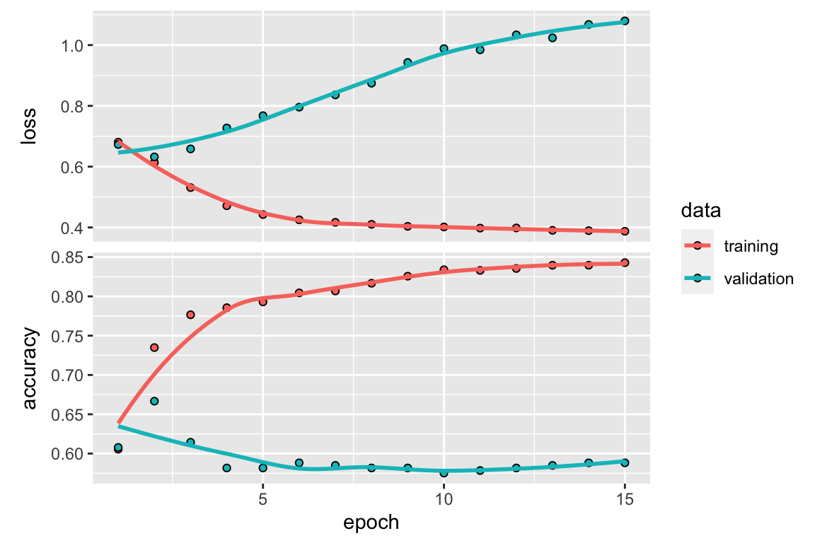
Figure 7.1: Validation data performance over multiple epochs in a MLP model
Figure 7.1 shows us how our validation data performs
as our MLP performs multiple feedforward/backpropagation epochs. Since we want to minimize our
validation data’s loss and maximize our validation data’s accuracy, we observe that out \(3\) epochs seems to be reasonable number of times to run our MLP
(note that this may change due to the issue mentioned above about random reproducibility in
keras).
set.seed(2)

mlp_model <- keras_model_sequential() %>%
  layer_dense(units = 8, activation = "relu", input_shape = c(num_features)) %>%
  layer_dense(units = 1, activation = "sigmoid")

mlp_model %>% compile(
  optimizer = "rmsprop",
  loss = "binary_crossentropy",
  metrics = c("accuracy")
)

mlp_model %>% keras::fit(x = dtm_train_matrix, y = train_targets_numerical,
                         epochs = 3, batch_size = 1)

mlp_results <- mlp_model %>% evaluate(x = dtm_test_matrix, test_targets_numerical)
mlp_results
## loss accuracy
## 0.5965526 0.6814622mlp_predicted_values <- mlp_model %>% predict_classes(dtm_test_matrix, batch_size = 1)
# confusion matrix
mlp_confusion_matrix <- caret::confusionMatrix(as.factor(mlp_predicted_values),
test_targets_categorical,
dnn = c("Predicted", "Actual"))
# confusion matrix table
mlp_confusion_matrix$table## Actual
## Predicted 0 1
## 0 116 53
## 1 69 145# around 70% accuracy
round(mlp_confusion_matrix$overall[1], 3) ## Accuracy
## 0.681# 95% CI
round(mlp_confusion_matrix$overall[3:4], 3) ## AccuracyLower AccuracyUpper
## 0.632 0.728Our MLP performs reasonably well with an accuracy of around \(70\%\) (and a 95% confidence interval around \([65\%, 75\%]\)).
7.3.2 Recurrent Neural Network
The keras package is used to fit a Recurrent Neural Network (RNN). Here, a RNN with
one input layer, one long short-term memory (LSTM)30 layer, and one output layer is created. The keras
requires features to be stored in matrices and targets to be numerical. Note that a RNN requires a
different type of DTM representation (as mentioned previously) where each word must be given a
unique numerical ID so that a sense of sequence can be maintained.
# the number of words to include in our vocab (keep the same as our other vocab)
vocab_size <- 806

# note that this tokenizer is based on the training data
rnn_tokenizer <- text_tokenizer(num_words = vocab_size) %>%
  fit_text_tokenizer(politifact_df_train$article_text)

train_sequences <- texts_to_sequences(rnn_tokenizer, politifact_df_train$article_text)
test_sequences <- texts_to_sequences(rnn_tokenizer, politifact_df_test$article_text)

# pad sequences (add 0's to the end) for documents that are short
rnn_x_train <-  pad_sequences(train_sequences, padding = "post")
rnn_x_test <- pad_sequences(test_sequences, padding = "post")

# take a look at what a RNN DTM looks like
rnn_x_train[1:5, 1:5]
## [,1] [,2] [,3] [,4] [,5]
## [1,] 57 48 146 165 3
## [2,] 53 135 0 0 0
## [3,] 219 136 9 368 414
## [4,] 1 11 15 415 0
## [5,] 1 485 137 573 98Now that we have our features in the right form (they have a notion of sequence), we can fit our RNN.
set.seed(2)

rnn_model <- keras_model_sequential()  %>%
  layer_embedding(input_dim = vocab_size, output_dim = 64) %>%
  layer_lstm(units = 128, dropout = 0.2, recurrent_dropout = 0.2) %>%
  layer_dense(units = 1, activation = "sigmoid")

rnn_model %>% compile(
  optimizer = "adam",
  loss = "binary_crossentropy",
  metrics = c("accuracy")
)

batch_size       <- 64
epochs           <- 15
validation_split <- 0.1

rnn_history <- rnn_model %>% keras::fit(
  rnn_x_train, train_targets_numerical,
  batch_size = batch_size,
  epochs = epochs,
  validation_split = validation_split
)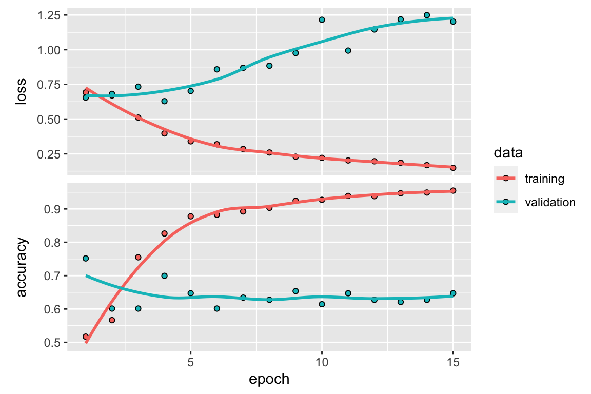
Figure 7.2: Validation data performance over multiple epochs in a RNN model
Figure 7.2 shows us how our validation data performs
as our RNN performs multiple feedforward/backpropagation epochs Since we want to minimize our
validation data’s loss and maximize our validation data’s accuracy, we observe that out \(3\) epochs seems to be reasonable number of times to run our MLP
(note that this may change due to the issue mentioned above about random reproducibility in
keras).
# recompile model
rnn_model <- keras_model_sequential()  %>%
  layer_embedding(input_dim = vocab_size, output_dim = 64) %>%
  layer_lstm(units = 128, dropout = 0.2, recurrent_dropout = 0.2) %>%
  layer_dense(units = 1, activation = "sigmoid")


rnn_model %>% compile(
  optimizer = "adam",
  loss = "binary_crossentropy",
  metrics = c("accuracy")
)

rnn_model %>% keras::fit(rnn_x_train, train_targets_numerical, epochs = 3, batch_size = batch_size)
rnn_results <- rnn_model %>% evaluate(rnn_x_test, test_targets_numerical)
rnn_predicted_values <- rnn_model %>% predict_classes(rnn_x_test, batch_size = batch_size)

# Confusion matrix
rnn_confusion_matrix <- caret::confusionMatrix(as.factor(rnn_predicted_values),
                                              test_targets_categorical,
                                              dnn = c("Predicted", "Actual"))

# confusion matrix table
rnn_confusion_matrix$table
## Actual
## Predicted 0 1
## 0 125 58
## 1 60 140# around 68% accuracy
round(rnn_confusion_matrix$overall[1], 3) ## Accuracy
## 0.692# 95% CI around (0.64, 0.73)
round(rnn_confusion_matrix$overall[3:4], 3) ## AccuracyLower AccuracyUpper
## 0.643 0.738Our RNN performs reasonably well with an accuracy of around \(68\%\) (and a 95% confidence interval around \([63\%, 73\%]\)).
-
“LSTMs were developed to deal with the vanishing gradient problem that can be encountered when training traditional RNNs.” “Long Short-Term Memory” (2020)↩︎